Note: This tutorial was generated from an IPython notebook that can be downloaded here.
Simulation PDFs
The time averaged joint PDFs from the TIGRESS simulations suites for all
7 models (see Simulation Model Tables) at all 4 heights are available. This
tutorial demonstrates how to download, read, and handle simulation PDFs
using TigressSimLoader class. More comphrensive examples can
be found at Figures in Paper II.
import twind
# read in simulated PDF
sim = twind.TigressSimLoader('R4','H')
sim.load(download=True)
Since TigressSimLoader is a child class of
TigressWindModel, this itself can be used to build model
PDFs. If the simulation pdf is passed in
TigressWindModel.set_axes() method, it will make axes identical
to the simulation PDF.
sim.set_axes(pdf=sim.simpdf,verbose=True)
modelpdf=sim.build_model()
Setting up from simulation PDF...
  u in (0.0,3.5) with du = 0.02
  w in (0.0,3.5) with dw = 0.02
  Sigma_SFR = 0.0917, ZISM = 0.0302
  Mpdf : cool=0.867 int=0.046 hot=0.085 total=0.998
  ppdf : cool=0.381 int=0.057 hot=0.560 total=0.999
  Epdf : cool=0.044 int=0.018 hot=0.938 total=1.000
  Zpdf : cool=0.824 int=0.047 hot=0.127 total=0.998
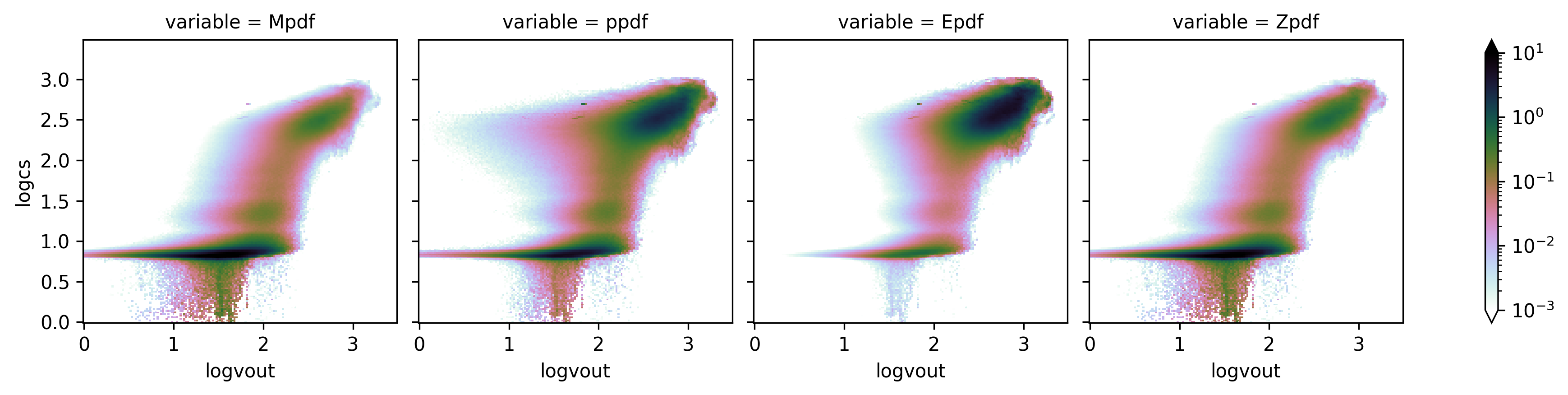
# show all PDFs from R4 simulation
simpdf = sim.simpdf
simpdf[['Mpdf','ppdf','Epdf','Zpdf']].to_array().plot(col='variable',
norm=LogNorm(vmin=1.e-3,vmax=10),
cmap=plt.cm.cubehelix_r)
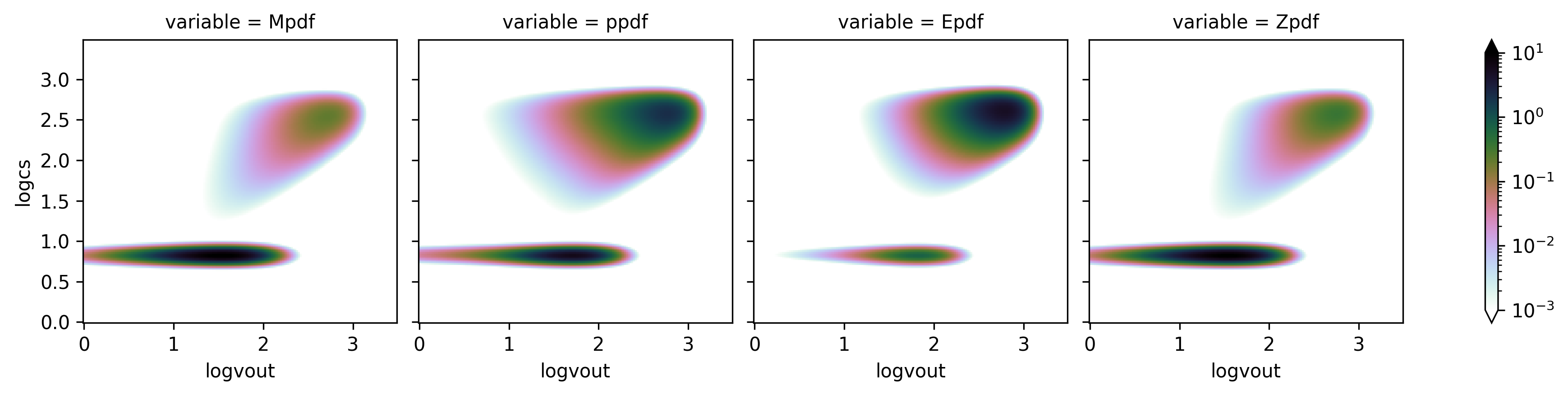
# this can be compared with model PDF
modelpdf[['Mpdf','ppdf','Epdf','Zpdf']].to_array().plot(col='variable',
norm=LogNorm(vmin=1.e-3,vmax=10),
cmap=plt.cm.cubehelix_r)
<xarray.plot.facetgrid.FacetGrid at 0x7fa83075e048>
Looking for more comprehensive comparisons? Check Figures in Paper II