Note: This tutorial was generated from an IPython notebook that can be downloaded here.
Particle Sampling
The TigressWindSampler class is a child class of the
TigressWindModel class. For sampling, it won’t build pdf
models, but use the scaling relations and parameters of the model.
import twind

sampler=twind.TigressWindSampler()
Sampling at a single epoch
For this example, we use
- \(\Sigma_{\rm SFR} = 10^{-2} M_\odot{\rm kpc^{-2} yr^{-1}}\),
- area = \(1 {\rm kpc}^2\)
- dt = 1 Myr
and
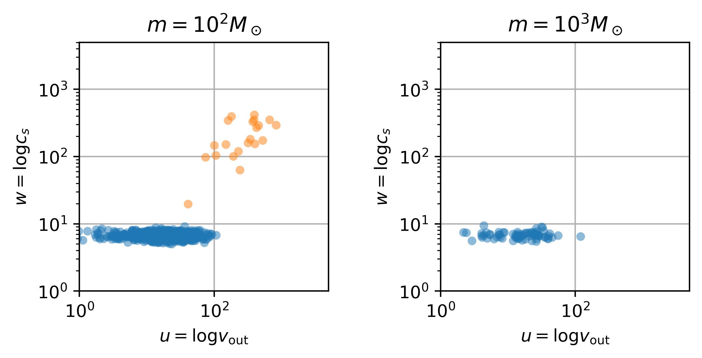
- \(m^{\rm cool} = m^{\rm hot} \in (10^2, 10^3)M_\odot\)
def draw_particle_dist(sfr0,area,dt,masses=[1.e2,1.e3,1.e4]):
    Nm=len(masses)
    fig, axes = plt.subplots(1,Nm,figsize=(3*Nm,3))

    for ax, m in zip(axes,masses):

        cool,hot=sampler.draw_mass(sfr0,m,m,area=area,dt=dt)

        plt.sca(ax)

        plt.plot(cool['vz'],cool['cs'],marker='o',ls='',ms=5,alpha=0.5,mew=0)
        plt.plot(hot['vz'],hot['cs'],marker='o',ls='',ms=5,alpha=0.5,mew=0)

        plt.xscale('log')
        plt.yscale('log')
        plt.title(r'$m = 10^{:.0f} M_\odot$'.format(np.log10(m)))
        ax.grid('on')
        ax.set_aspect('equal')
        plt.xlim(1.,5.e3)
        plt.ylim(1.,5.e3)
        plt.xlabel(r'$u=\log v_{\rm out}$')
        plt.ylabel(r'$w=\log c_s$')
        plt.tight_layout()
    return fig
sfr0 = 1.e-2
area = 1
dt = 1.e6

f = draw_particle_dist(sfr0,area,dt,masses=[1.e2,1.e3])
The mass in the outflow can be obatined by
For a chosen \(\Sigma_{\rm SFR}\), the total, cool, and hot mass loading factors are
etaM=sampler._eta_sfr_scaling(sfr0,'M_total')
etaMc=sampler._eta_sfr_scaling(sfr0,'M_cool')
etaMh=sampler._eta_sfr_scaling(sfr0,'M_hot')
print('eta_M={:.2f} eta_M^cool={:.2f} eta_M^hot={:.2f}'.format(etaM, etaMc, etaMh))
eta_M=7.07 eta_M^cool=6.54 eta_M^hot=0.19
which give the outflowing mass in each phase
print('M_out={:.3g} M_out^cool={:.3g} M_out^hot={:.3g}'.format(etaM*sfr0*area*dt,etaMc*sfr0*area*dt,etaMh*sfr0*area*dt))
M_out=7.07e+04 M_out^cool=6.54e+04 M_out^hot=1.93e+03
Therefore, even for \(m^{\rm hot}=10^3 M_\odot\), we expect to sample a few particles as shown in the right panel of the above figure.
Sampling from a time series
For this example, we use a sinusoidal function for SFR surface density time series for 200 Myr with
- mean \(\Sigma_{\rm SFR} = 10^{-3} M_\odot{\rm kpc^{-2} yr^{-1}}\),
- period of 50 Myr
tmax = 2.e8
dt = 1.e6
time = np.arange(0,tmax,dt)
tp = 5.e7
sfr0 = 2.e-3
area = 1

sfr=sfr0*0.5*(np.sin(2*np.pi/tp*time)+2)
For a given time series of \(\Sigma_{\rm SFR}\), we get reference values of outflow rates using the scaling relations of outflow loading factors (of each outflow phase) presented in Kim et al. (2020a).
The TigressWindSampler.get_refs() method returns four lists
containing time series of reference outflow rates and loading factors
for total, cool, and hot outflows. Each list contains mass,
momemtum, energy, and metal in order.
refs,eta,etac,etah = sampler.get_refs(sfr)
mout = [eta[0]*refs[0]*area*dt, etac[0]*refs[0]*area*dt, etah[0]*refs[0]*area*dt]
Eout = [eta[2]*refs[2]*area*dt, etac[2]*refs[2]*area*dt, etah[2]*refs[2]*area*dt]
print('mean outflowing mass = {:.3g} (total) {:.3g} (cool)  {:.3g} (hot) Msun'.format(mout[0].mean(),mout[1].mean(),mout[2].mean()))
print('mean outflowing energy = {:.3g} (total) {:.3g} (cool) {:.3g} (hot) erg'.format(Eout[0].mean(),Eout[1].mean(),Eout[2].mean()))
mean outflowing mass = 2.73e+04 (total) 2.62e+04 (cool)  429 (hot) Msun
mean outflowing energy = 2.16e+51 (total) 4.3e+50 (cool) 1.82e+51 (hot) erg
For the area of 1 kpc\(^2\) and time interval 1 Myr considered here, we expect the mean mass and energy in outflow are \(2.7\times10^4 M_\odot\) and \(2.2\times10^{51}\) erg, respectively. The mass ratio between cool and hot outflows is about 50, therefore, for a fair sampling, we might need \(m^{\rm cool}/m^{\rm hot}\sim50\) with \(m^{\rm cool}<10^4 M_\odot\).
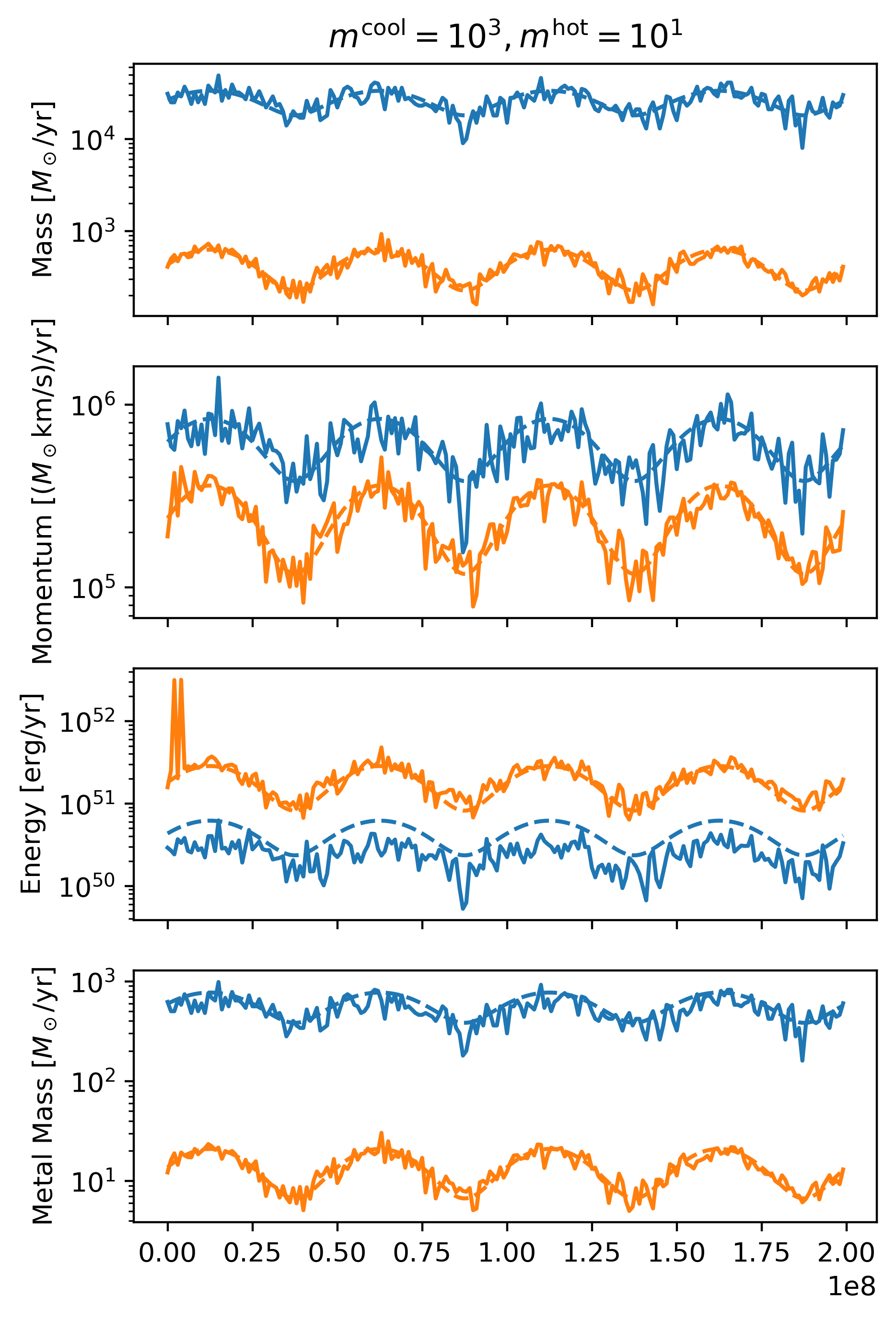
Frist, as a well sampled example, we use
- \(m^{\rm cool} = 10^3 M_\odot\)
- \(m^{\rm hot} = 10^1 M_\odot\)
def draw_particle_time_series(time, sfr, mc, mh, area, dt):
    refs,eta,etac,etah = sampler.get_refs(sfr)
    cool,hot=sampler.draw_mass(sfr,mc,mh,area=area,dt=dt)

    fig,axes = plt.subplots(4,1,sharex=True,figsize=(5,8))
    for p, etas_ in zip([cool,hot],[etac,etah]):
        outs=twind.to_time_series(p,time)

        for ax, q, qref, eta in zip(axes,outs,refs,etas_):
            plt.sca(ax)
            l,=plt.plot(time,q)
            plt.plot(time,eta*qref*area*dt,color=l.get_color(),ls='--')
            plt.yscale('log')

    axes[0].set_title(r'$m^{{\rm cool}} = 10^{}, m^{{\rm hot}} = 10^{}$'.format(int(np.log10(mc)),int(np.log10(mh))))
    axes[0].set_ylabel(r'Mass $[M_\odot/{\rm yr}]$')
    axes[1].set_ylabel(r'Momentum $[(M_\odot {\rm km/s})/{\rm yr}]$')
    axes[2].set_ylabel(r'Energy $[{\rm erg/yr}]$')
    axes[3].set_ylabel(r'Metal Mass $[M_\odot/{\rm yr}]$')
    return fig
Here, a utility function to_time_series() is used to convert
particle data into time series of rates.
f = draw_particle_time_series(time, sfr, 1.e3, 1.e1, area, dt)
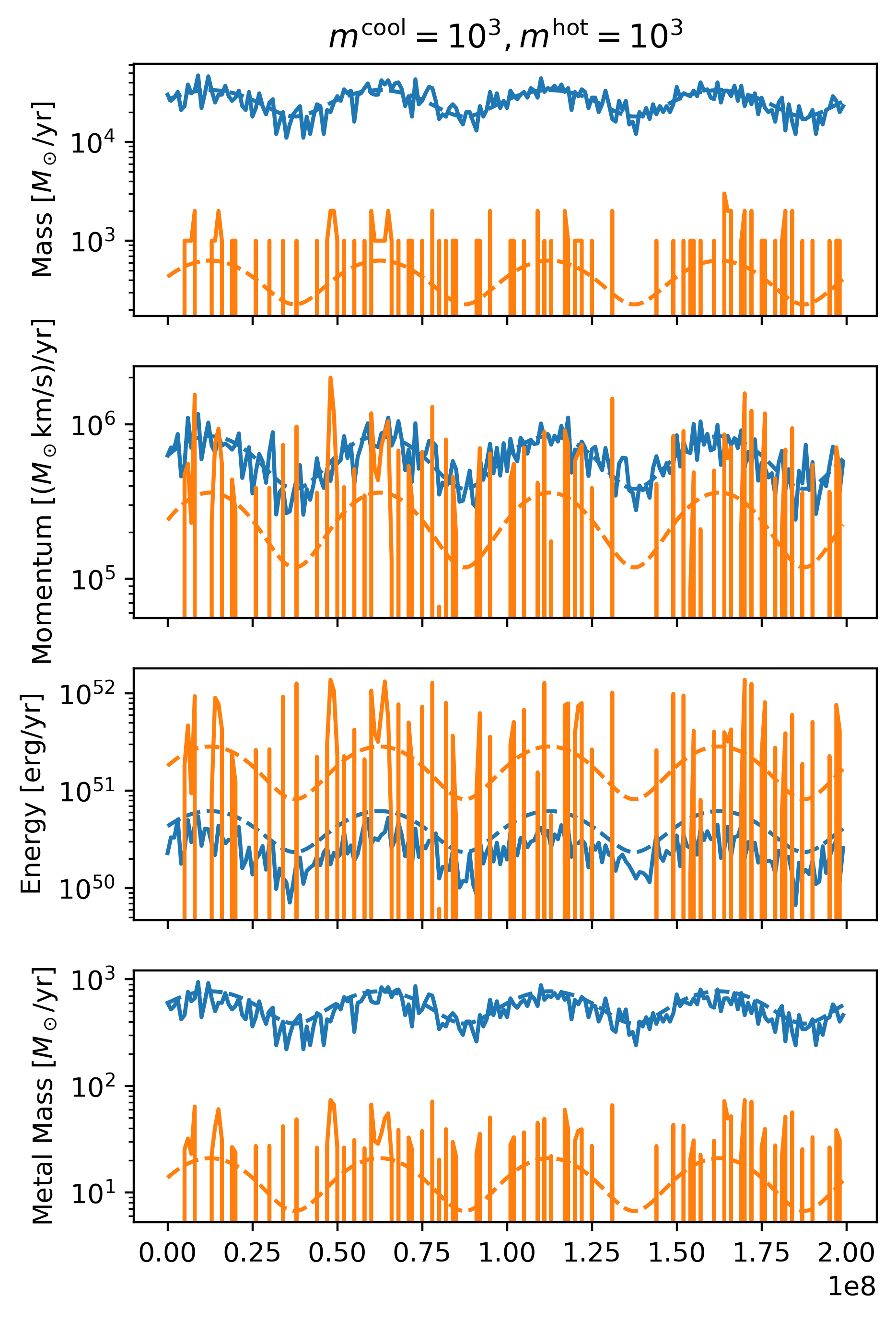
The second example is for well sampled cool phase but poorly sampled hot phase.
- \(m^{\rm cool} = 10^3 M_\odot\)
- \(m^{\rm hot} = 10^3 M_\odot\)
f = draw_particle_time_series(time, sfr, 1.e3, 1.e3, area, dt)