Note: This tutorial was generated from an IPython notebook that can be downloaded here.
Loading Factors from 3D PDFs
See Quickstart for details of the first step. For this tutorial, we use the default ranges for axes setup.
import twind

tw=twind.TigressWindModel(z0='H',verbose=False)
tw.set_axes(verbose=True)
cs: min=0, max=4, N=500
vout: min=0, max=4, N=500
sfr: min=-6, max=2, N=100
Now we build joint PDFs as a function of SFR surface density, which gives a 3D PDF model.
pdf=tw.build_model(renormalize=True,energy_bias=True,verbose=False)
Note
After building the 3D PDF model, all subsequent manipulations heavily rely on the functionalities of xarray. We only show a few examples here.
Slicing back to 2D PDF
xarray.Dataset provides very useful functionality for slicing and
interpolating through a method sel. Since we build a 3D PDF on the
decretized sfr array, to get a PDF with a particular choice of
sfr using the current 3D PDF, we would want either get the PDF with
the closet value of sfr or interpolate to the chosen sfr. This
can be done very easily with xarray.
# find the nearest one
pdf_nearest=pdf.sel(logsfr=-2, method='nearest')

# intepolate; this takes longer
pdf_interp=pdf.interp(logsfr=-2)

print('log sfr:{} {}'.format(pdf_nearest.logsfr.data,pdf_interp.logsfr.data))
log sfr:-2.04040404040404 -2
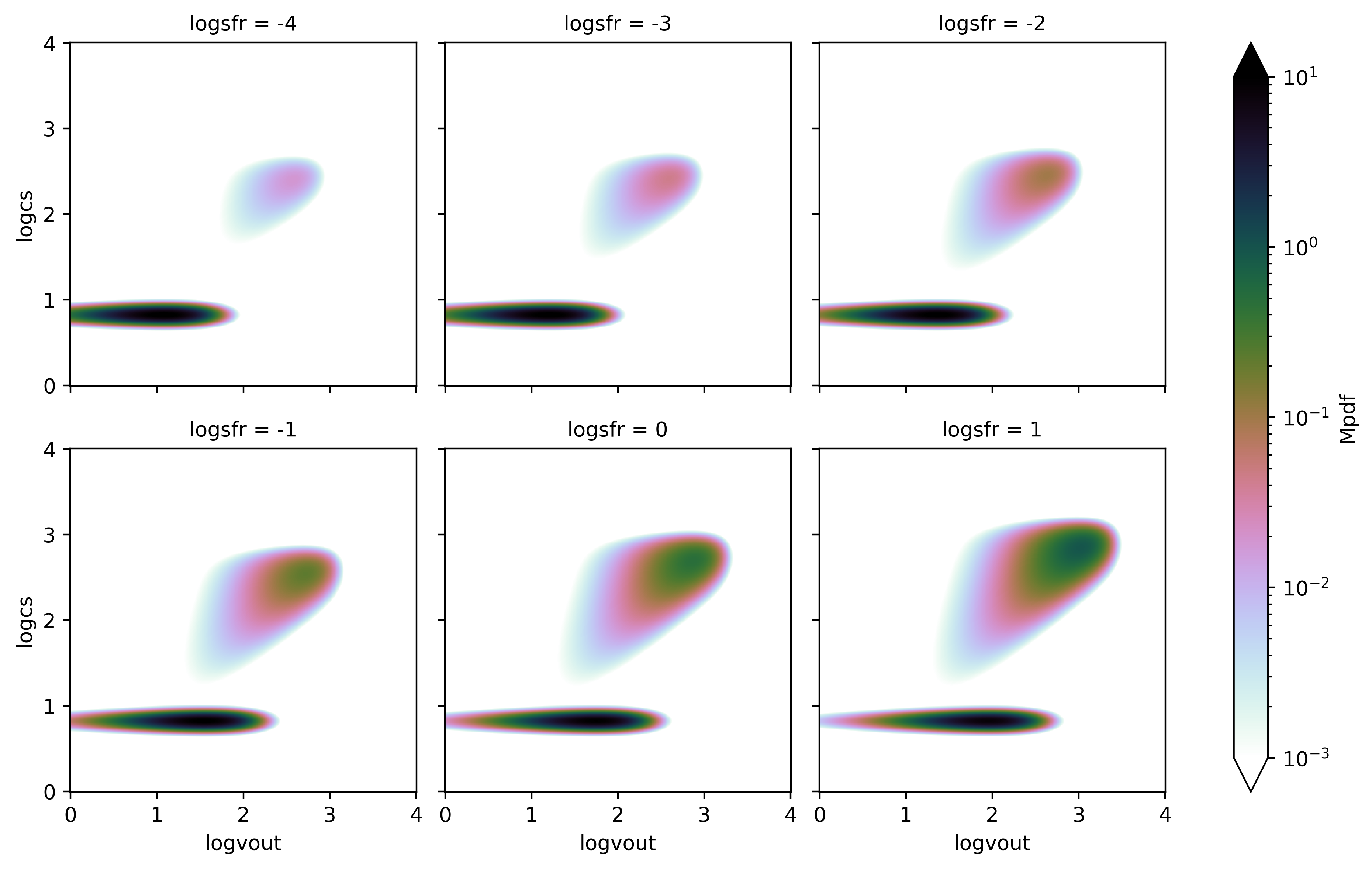
Interpolation (or slicing) within the range of sfr would be useful
to compare pdfs at different SFRs quickly.
g=pdf['Mpdf'].interp(logsfr=[-4,-3,-2,-1,0,1]).plot(col='logsfr',col_wrap=3,
                                                    norm=LogNorm(vmin=1.e-3,vmax=10),
                                                    cmap=plt.cm.cubehelix_r
                                                   )
Selecting escapable outflows: constant velocity cut
For a practical use, we may want to select outflows with a certain velocity (or Bernoulli velocity) cut given a halo escape velocity. Here’s how to do this.
We may first want to calculate the cumulative distribution functions
(CDF) with vBz > vBzcut. We then obtain the loading factors of
selected gas by multiplying the total loading factors, which are stored
as etaM, etap, etaE, etaZ in the original Dataset.
dbinsq=pdf.attrs['dlogcs']*pdf.attrs['dlogvout']
pdfs=['Mpdf','Mpdf-cool','Mpdf-hot',
'ppdf','ppdf-cool','ppdf-hot',
'Epdf','Epdf-cool','Epdf-hot',
'Zpdf','Zpdf-cool','Zpdf-hot',]
sfr=10.**pdf['logsfr']
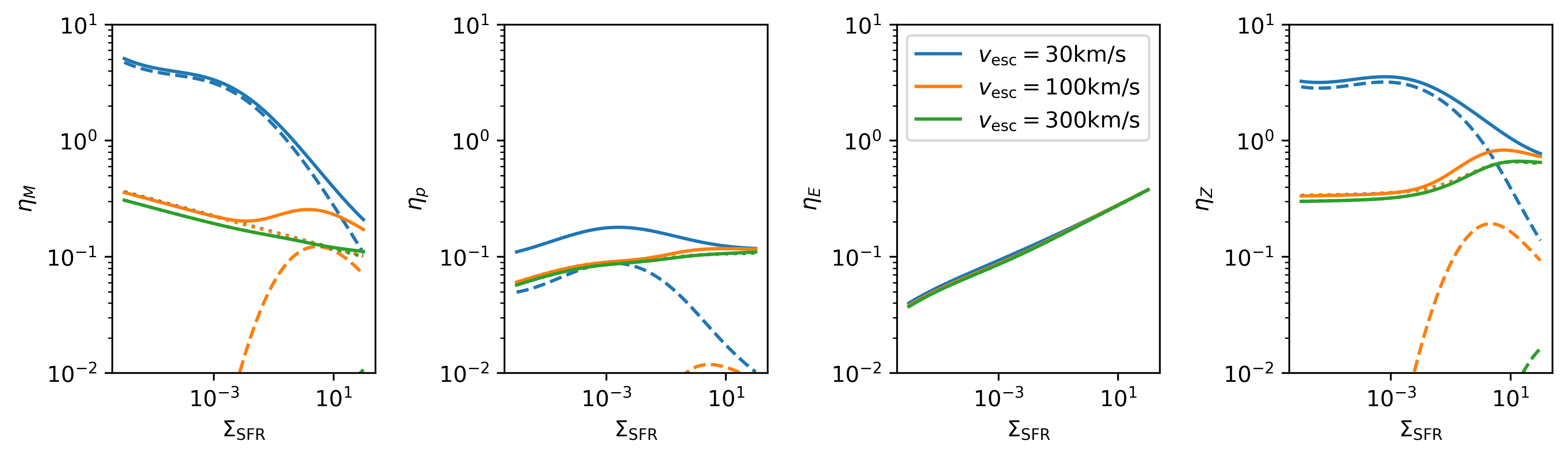
# For a constant velocity cut
fig, axes = plt.subplots(1,4,figsize=(10,3))
for vBzcut0 in [30,100,300]:
cdf=pdf[pdfs].where(pdf['vBz']>vBzcut0).sum(dim=['logcs','logvout'])*dbinsq
for ax,q in zip(axes.flat,['M','p','E','Z']):
plt.sca(ax)
eta=pdf['eta'+q]
l,=plt.plot(sfr,cdf[q+'pdf']*eta,label=r'$v_{{\rm esc}}={}{{\rm km/s}}$'.format(vBzcut0))
plt.plot(sfr,cdf[q+'pdf-cool']*eta,ls='--',color=l.get_color())
plt.plot(sfr,cdf[q+'pdf-hot']*eta,ls=':',color=l.get_color())
plt.ylabel(r'$\eta_{}$'.format(q))
plt.xlabel(r'$\Sigma_{\rm SFR}$')
axes[2].legend()
plt.setp(axes,'xscale','log')
plt.setp(axes,'yscale','log')
plt.setp(axes,'ylim',(1.e-2,1.e1))
plt.tight_layout()
Note
\(\Sigma_{\rm SFR}\) is in \(M_\odot{\rm kpc^{-2} yr^{-1}}\) everywhere in this document.
The mass (and metal) loading factor \(\eta_M\) changes dramatically as different velocity cuts are applied. This is because the cool outflow carries most of mass (shown as dashed lines), which has typical outflow velocities insufficient to escape for \(v_{\rm esc}>100 {\rm km/s}\). However, at very high \(\Sigma_{\rm SFR}\), cold outflow may contribute to the mass outflow rate significantly again, while one should take this with a grain of salt since those are outside our original parameter space \(10^{-4}<\Sigma_{\rm SFR}<1\) over which the model is calibrated. On the other hand, the energy loading factor \(\eta_E\) is unchaged since it is dominated by the hot outflow whose Bernoulli velocity is already larger than 300km/s even at low \(\Sigma_{\rm SFR}\).
Selecting escapable outflows: SFR-dependent velocity cut
For some reasons, if the escape velocity is a function of SFR surface
density, we get loading factors with a varying vBzcut easily using
xarray.Dataset.where as it correctly broadcasts the information.
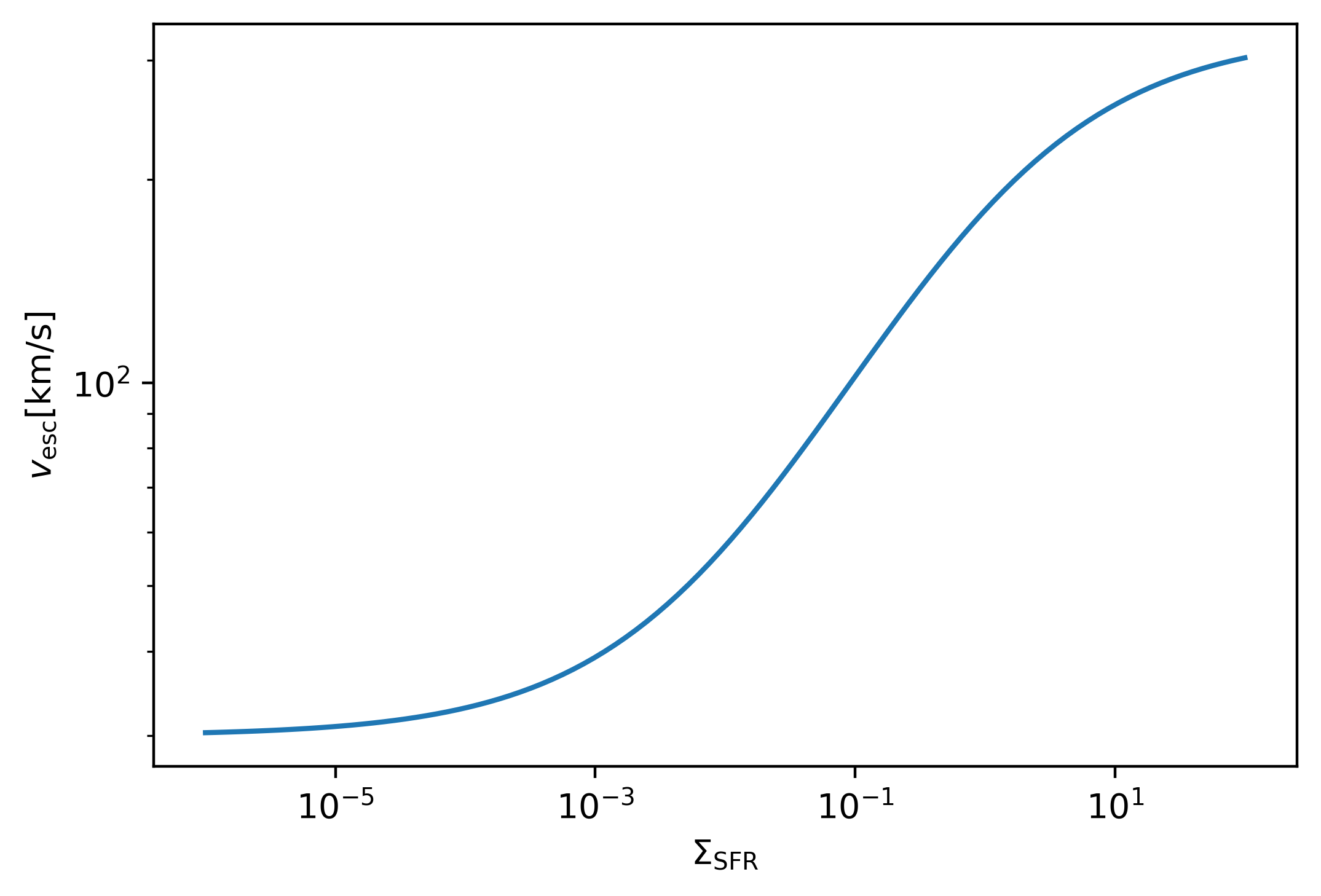
Let’s assume a particular form of the escape velocity:
vBzcut = 300.*sfr**0.5/(sfr**0.5+1)+30
plt.loglog(sfr,vBzcut)
plt.xlabel(r'$\Sigma_{\rm SFR}$');
plt.ylabel(r'$v_{\rm esc} [{\rm km/s}]$');
fig, axes = plt.subplots(1,4,figsize=(10,3))

for vBzcut0 in [30,100,300]:
    cdf=pdf[pdfs].where(pdf['vBz']>vBzcut0).sum(dim=['logcs','logvout'])*dbinsq
    for ax,q in zip(axes.flat,['M','p','E','Z']):
        plt.sca(ax)
        eta=pdf['eta'+q]
        l,=plt.plot(sfr,cdf[q+'pdf']*eta,lw=1)
        plt.plot(sfr,cdf[q+'pdf-cool']*eta,ls='--',color=l.get_color(),lw=1)
        plt.plot(sfr,cdf[q+'pdf-hot']*eta,ls=':',color=l.get_color(),lw=1)
        plt.ylabel(r'$\eta_{}$'.format(q))
        plt.xlabel(r'$\Sigma_{\rm SFR}$')

cdf=pdf[pdfs].where(pdf['vBz']>vBzcut).sum(dim=['logcs','logvout'])*dbinsq
for ax,q in zip(axes.flat,['M','p','E','Z']):
    plt.sca(ax)
    eta=pdf['eta'+q]
    l,=plt.plot(sfr,cdf[q+'pdf']*eta,label='total',lw=2)
    plt.plot(sfr,cdf[q+'pdf-cool']*eta,ls='--',color=l.get_color(),label='cool',lw=2)
    plt.plot(sfr,cdf[q+'pdf-hot']*eta,ls=':',color=l.get_color(),label='hot',lw=2)
    plt.ylabel(r'$\eta_{}$'.format(q))
    plt.xlabel(r'$\Sigma_{\rm SFR}$')
axes[2].legend()

plt.setp(axes,'xscale','log')
plt.setp(axes,'yscale','log')
plt.setp(axes,'ylim',(1.e-2,1.e1))
plt.tight_layout()
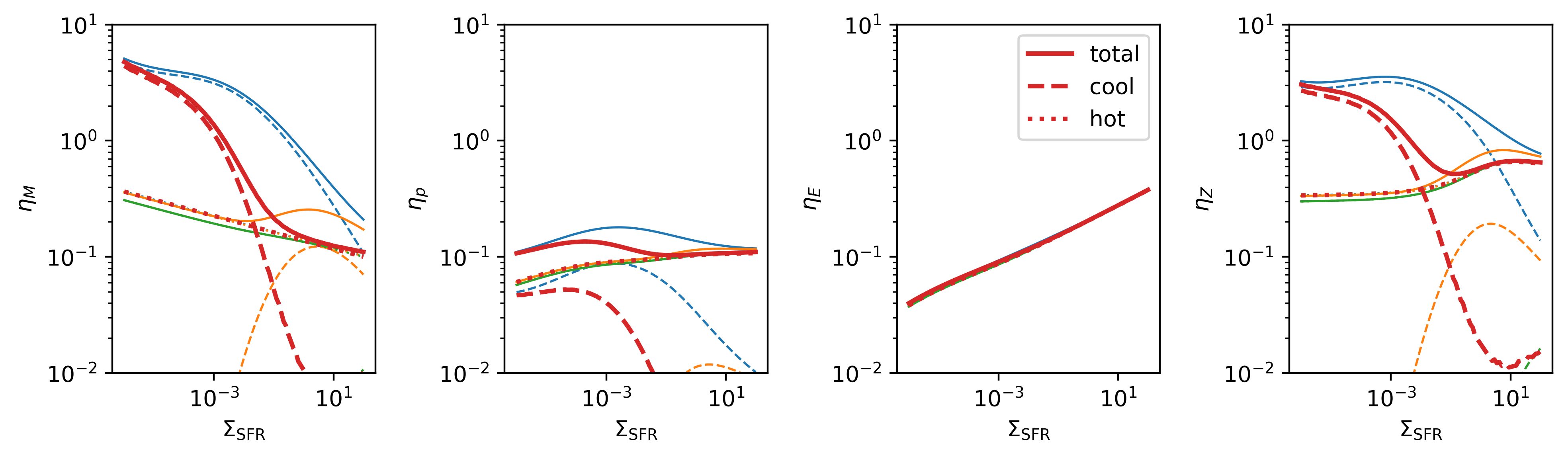
Obviously, the result (red) falls between vBzcut0=30 (blue) and
vBzcut0=300 (green) cases.