Note: This tutorial was generated from an IPython notebook that can be downloaded here.
Quickstart
Step 1: initialize Twind class
We are initilizing the TigressWindModel class with default
parameters set to match the TIGRESS simulation suite results at
\(|z|=H\) (see Simulation PDFs). Possible options are
z0=['H', '2H', '500', '1000'].
import twind

tw=twind.TigressWindModel(z0='H',verbose=True)
number of wind phase = 2
galactic parameter = sfr
reference height = H
cool_params
    A_v = 2.302585092994046
    p_v = 1
    d_v = 2
    A_cs = 9.185985478173896
    cs0 = 6.7
    sigma = 0.1
    vout0 = 25.0
hot_params
    A_vB = 5.196378098798331
    p_vB = 4
    d_vB = 2
    A_M = 1.151292546497023
    Mach0 = 0.5
    p_M = 1
    d_M = 3
params
    Esn = 1e+51 erg
    mstar = 95.5 solMass
    vcool = 200.0 km / s
    Mej = 10.0 solMass
    ZSN = 0.2
    ZISM0 = 0.02
    vej = 3171.4804794827423 km / s
ref_params
    Mref = 95.5 solMass
    pref = 2.5e+48 erg s / km
    Eref = 1e+51 erg
    Zref = 2.0 solMass
scaling_params
    a = [-0.067 -1.216 -0.857  0.013 -1.426 -2.151 -1.013 -0.879 -2.228 -2.627
 -0.698 -0.695  0.171 -0.942 -0.375  0.281]
    b = [-0.441 -0.227 -0.069 -0.418 -0.287 -0.149  0.016 -0.157 -0.117 -0.076
  0.136  0.108 -0.364 -0.146  0.04  -0.335]
    A = [0.86 0.06 0.14 1.03 0.04 0.01 0.1  0.13 0.01 0.   0.2  0.2  1.48 0.11
 0.42 1.91]
    p = [0.559 0.773 0.931 0.582 0.713 0.851 1.016 0.843 0.883 0.924 1.136 1.108
 0.636 0.854 1.04  0.665]
With the verbose=True option, key attributes are printed.
cool_params: parameters for cool mass loading PDF. See Joint PDF Modelhot_params: parameters for hot mass loading PDF. See Joint PDF Modelparams: other physical parameters related to the particular choices of the TIGRESS simulation suite (see Kim et al. (2020a))ref_params: outflow rates are normalized by \(\Sigma_{\rm SFR}q_{\rm ref}/m_*\) to obtain loading factorsscaling_params: fitting results for velocity-integrated loading factors as a function of SFR surface density (in log-log space) presented in Kim et al. (2020a). Each array contains the results for four loading factors (mass, momentum, energy, metal) of four phases (cool, intermediate, hot, whole). E.g., first four values are the results for the mass loading factor of cool, intermediate, hot, and whole gas.ais the interceptbis the slopeAis \(10^a\)pis \(b+1\) for flux scalings.
Note
\(\Sigma_{\rm SFR}\) is in \(M_\odot{\rm kpc^{-2} yr^{-1}}\) everywhere in this document.
Note
\(u \equiv \log v_{\rm out}\) and \(w \equiv \log c_s\) as defined in Kim et al. (2020b).
Step 2: setup axes
We use xarray extensibly for easier manipulation with broadcasting, indexing, slicing, and interpolation.
The TigressWindModel.set_axes() method accept either the
simulated PDF (in the form of xarray.Dataset) or list of ranges (in
log) and number of bins for vout and cs axes (sfr can either
be a scalar or an array). Default is
vout= (0,4,500)cs= (0,4,500)sfr= (-6,2,100)
This function will set attributes u=logvout and w=logcs as 1D
DataArray as well as vBz and Mach as 2D DataArray for
future use. If a range of sfr is passed, it will also set a member
logsfr as 1D DataArray with different coordinates so that the
final PDFs would be 3D DataArray.
For this example, we use a single value of SFR surface density and reduced number of bins for velocity axes.
tw.set_axes(vout=(0,4,200),cs=(0,4,200),sfr=0.01,verbose=True)
sfr=0.01
cs: min=0, max=4, N=200
vout: min=0, max=4, N=200
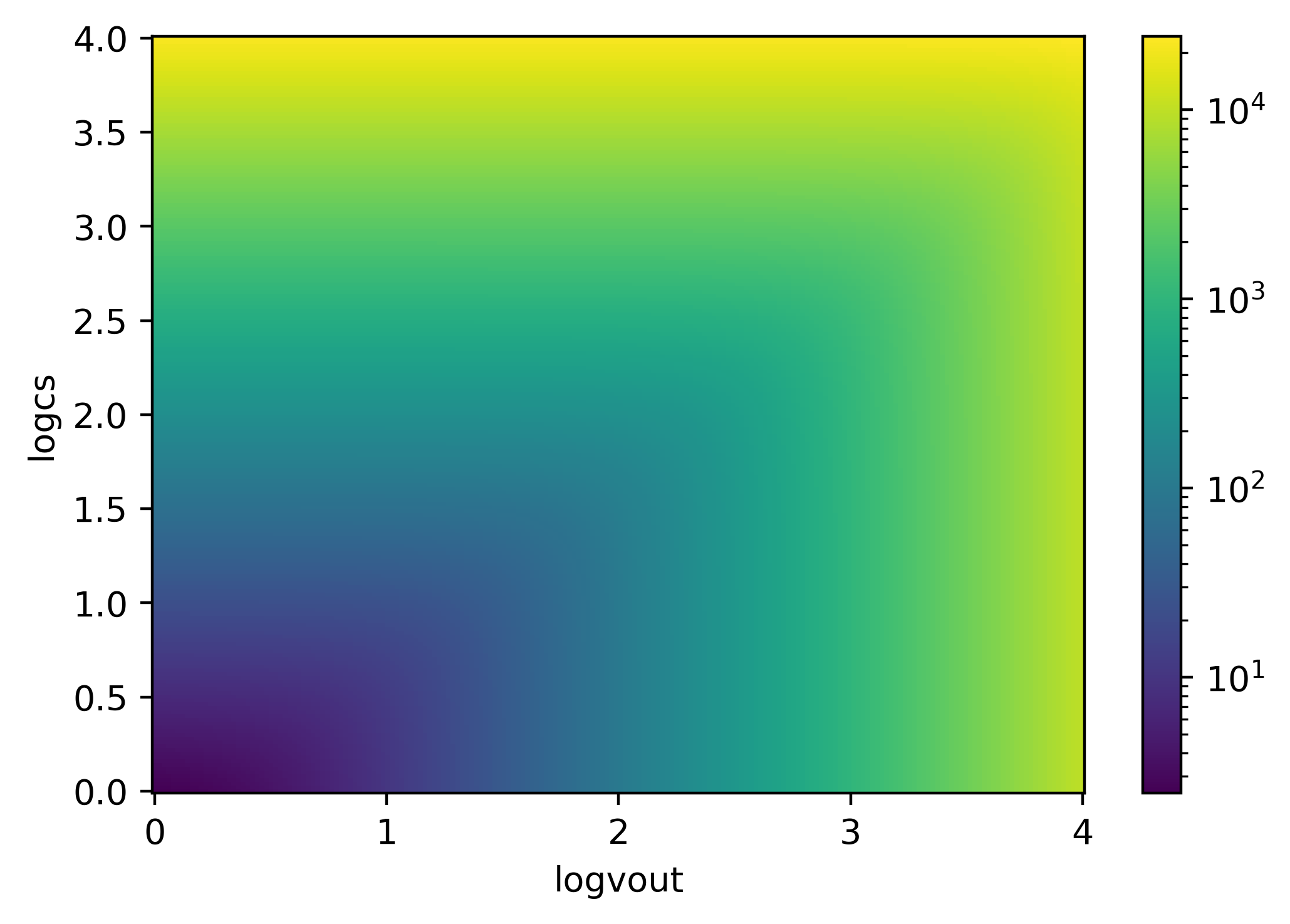
We make sure that vBz and Mach are 2D while u=logvout and
w=logcs are 1D.
print('u shpae:',tw.u.shape)
print('w shape:',tw.w.shape)
print('vBz shpae:',tw.vBz.shape)
print('Mach shape:',tw.Mach.shape)
g=tw.vBz.plot(norm=LogNorm())
u shpae: (200,)
w shape: (200,)
vBz shpae: (200, 200)
Mach shape: (200, 200)
Step 3: build mass loading PDFs
We have a method TigressWindModel.build_Mpdf() that
automatically builds model PDFs for mass loading factor and return a
xarray.Dataset. Note that if the range of (u,w) is not large
enough, the mass PDF may not integrate to 1 (use verbose=True to
check this).
Depending on the choice of the sfr axis, the resulting PDF can
either be 2D or 3D. The returned Dataset have variables for PDFs
(Mpdf, Mpdf-cool, Mpdf-hot) for total, cool, and
hot outflow components. This also contains vBz and Mach as
2D arrays for convenience. In addition, the integrated loading factor
(etaM and their phase-separated values, i.e., etaM-cool and
etaM-hot) as a function of sfr are saved. If sfr is a
scalar, these are also scalars.
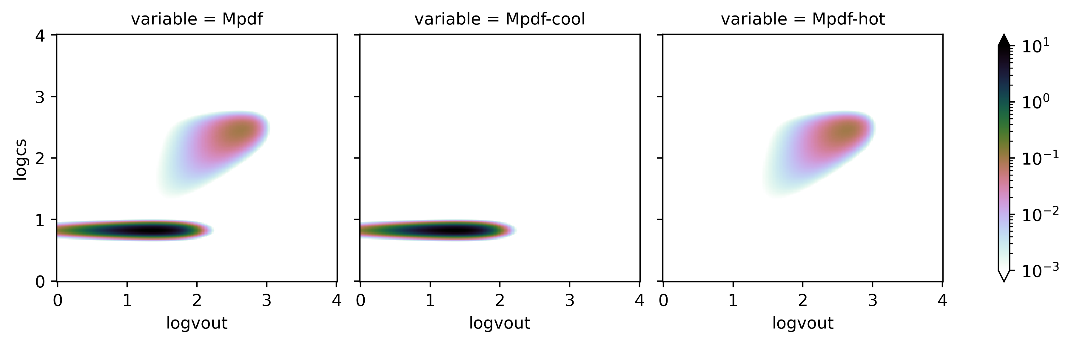
pdf = tw.build_Mpdf(verbose=True)
Mass PDFs are integrated to: cool=0.997 hot=1
pdf[['Mpdf','Mpdf-cool','Mpdf-hot']].to_array().plot(col='variable',
                                                   norm=LogNorm(vmin=1.e-3,vmax=10),
                                                   cmap=plt.cm.cubehelix_r
                                                  )
<xarray.plot.facetgrid.FacetGrid at 0x7f88b069a400>
Step 4: build all PDFs
We have a method TigressWindModel.build_model() that
automatically builds model PDFs for mass, momentum, energy, and metal
loading factors and return a xarray.Dataset containing all. The last
three PDFs are reconstructed from the mass PDF as outlined in Kim et
al. (2020b). By default, they are renormalized to ensure the
integration over the entire (u,w) gives 1. Note that the metal PDF
is not normalized for the input ZISM but for ZISM0.
Again, depending on the choice of the sfr axis, the resulting PDFs
can either be 2D or 3D. The returned Dataset have variables for PDFs
(Mpdf, ppdf, Epdf, Zpdf) and their phase-separated
counterparts (e.g., Mpdf-cool, Mpdf-hot). The
velocity-integrated loading factors (etaM, etap, etaE,
etaZ) and their phase-separated counterparts (e.g., etaM-cool
and etaM-hot) as a function of sfr are also stored. Finally, if
renormalize=True (default), it also stores the renormalization
factors (p_renorm, E_renorm, Z_renorm), which are also a
function of sfr.
The Dataset has attributes for the choice of ZISM for the metal
loading PDF as well as the bin sizes dlogcs and dlogvout for
convenience.
pdf=tw.build_model(renormalize=True,energy_bias=True)
As it builds a model PDF, it automatically checks whether the mass PDFs are integrated to 1. I.e., both cool and hot PDFs should satisfy
individually. Again, this may depend on the (u,w) range. We then
apply loading factor ratios to combine the mass loading PDF as
Note that Mpdf-cool and Mpdf-hot (and corresponding other PDFs)
in the returned Dataset are not \(\tilde{f}_M^{\rm ph}\) but
\(\frac{\eta_M^{\rm ph}}{\eta_M}\tilde{f}_M^{\rm ph}\).
dudw=pdf.attrs['dlogvout']*pdf.attrs['dlogcs']
print('contribution to')
print('mass outflow rate from cool is {:.3f} and hot is {:.3f}'.format(
    pdf['Mpdf-cool'].sum().data*dudw,pdf['Mpdf-hot'].sum().data*dudw))
print('energy outflow rate from cool is {:.3f} and hot is {:.3f}'.format(
    pdf['Epdf-cool'].sum().data*dudw,pdf['Epdf-hot'].sum().data*dudw))
contribution to
mass outflow rate from cool is 0.968 and hot is 0.029
energy outflow rate from cool is 0.081 and hot is 0.919
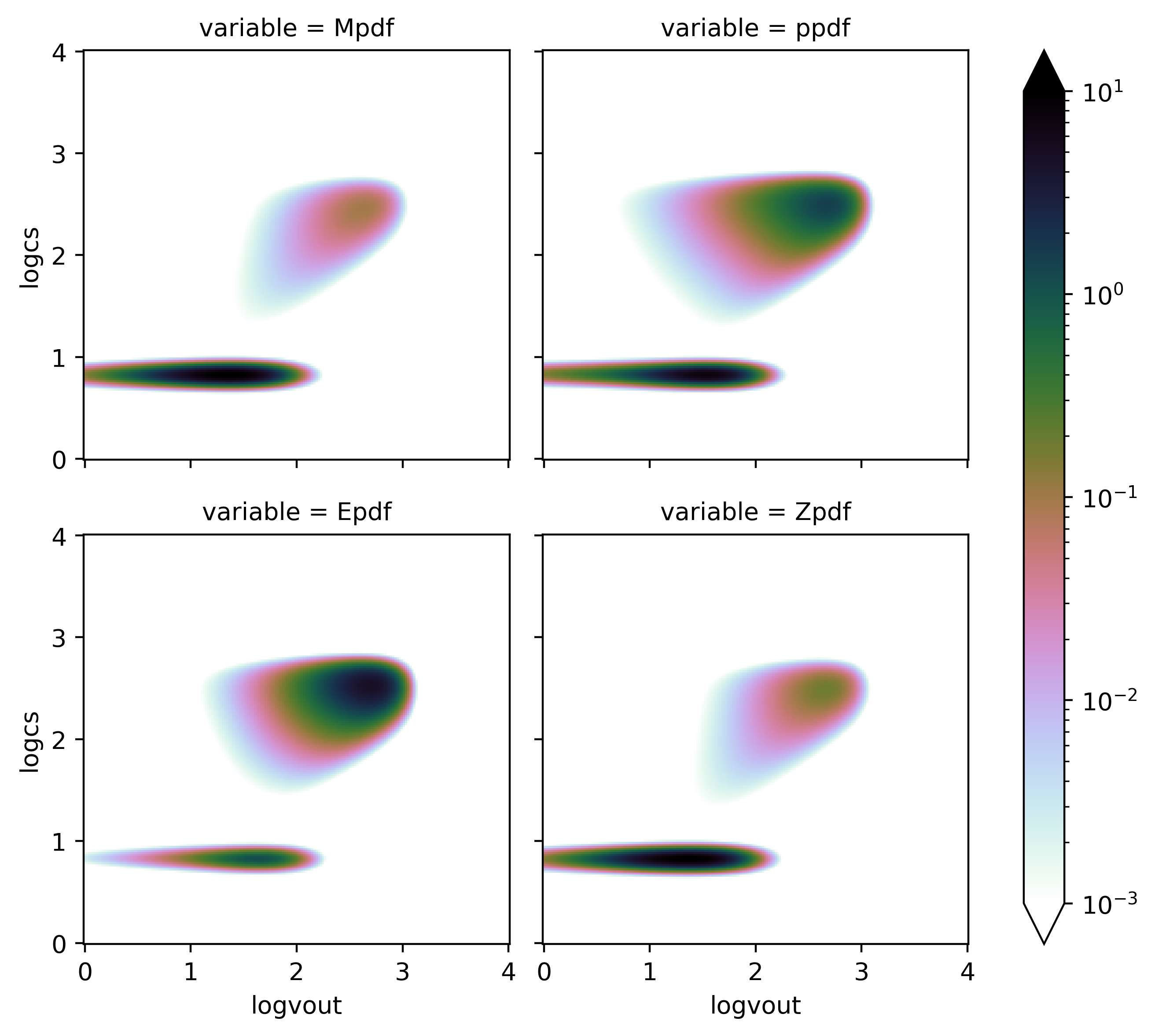
Finally, 2D PDFs for mass, momentum, energy, and metal loadings at \(\Sigma_{\rm SFR}=10^{-2}\) look as follows.
pdf[['Mpdf','ppdf','Epdf','Zpdf']].to_array().plot(col='variable',col_wrap=2,
                                                   norm=LogNorm(vmin=1.e-3,vmax=10),
                                                   cmap=plt.cm.cubehelix_r
                                                  )
<xarray.plot.facetgrid.FacetGrid at 0x7f8870725898>